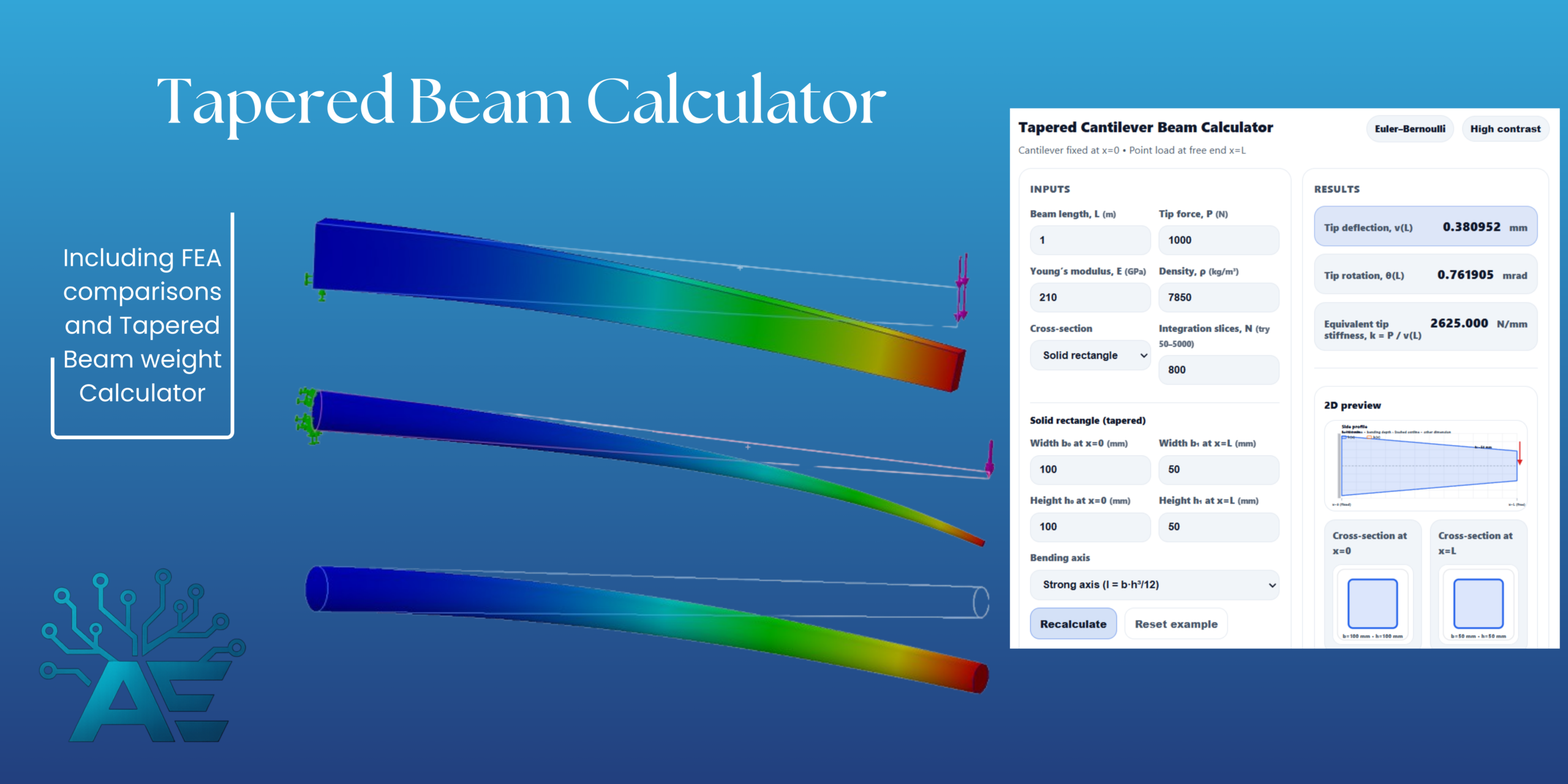
Calculations for a standard cantilever beam with a constant cross-section are straightforward and well-supported by standard formulas. However, when a taper is introduced, the complexity of determining volume and tip displacement increases significantly. I observed a consistent demand for a more accessible way to handle these scenarios—specifically for calculating weight based on material density and predicting tip deflection.

To provide an efficient solution, I developed a Tapered Beam Calculator designed for rapid estimation.

While this calculator is designed to be a quick and user-friendly tool, it remains an approximation. To understand its performance and limitations, I have compared the results against Finite Element Method (FEM) analysis.

The situation is the following. A simple Cantilever beam with a force in the end. Normally a cross-section of this beam that is constant throughout the length is easy to calculate, and has standard formulas, but for a tapered beam it is different. Here it is not exactly trivial what to do, and therefore this calculator is made.

Select your preferred unit system (Metric/Imperial) using the toggle in the top-right corner.

How to use the tapered beam calculator

Whether you want to find the weight of your tapered beam or the deflection, then this calculator can do it.

The first things you need to input is your beam length in meters, the tip force P in Newton. Young’s modulus for your material in GPa, and the density of your material in kg/m^3

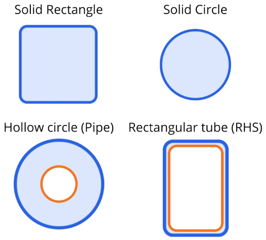
Then you need to select which cross section you have.

I implemented 4 types of cross section which can be seen here:

Then you need to select what amount of integration slices you want. This is because we are evaluting an integral numerically which we will get to later. This increase accuracy of the numerical method (Midpoint rule) the more slices we have. So you can try out different values and see how the results changes.

Then for the different cross section i need you to enter the dimensions.

For the solid tapered rectangle you need to input the width and height dimensions of x=0 and x=L.

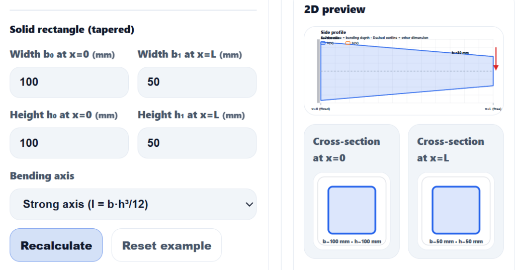
In the calculator i assume a linear tapering for all cross section, and if your problem that you are trying to solve, does not have a linear tapering, then i recommend going directly into an FEA tool like Solidworks or Ansys to solve the problem. And that is because analytical methods become very difficult and time consuming compared to just using FEA if you have difficult geometry.

Worst cases it is simply just impossible to calculate analytically.

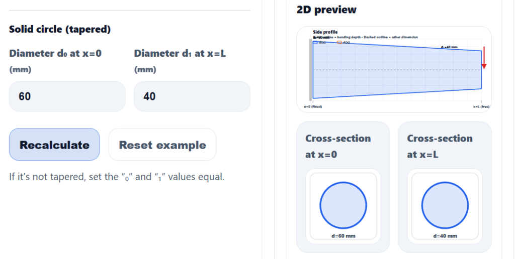
For the Solid circle it is easy. Simply just input the diameter at x=0 and x=L respectively

For the Hollow circle you input basically the same, but with one adjustment which is the Wall thickness aswell.

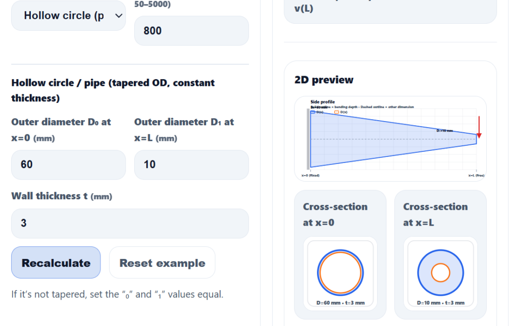
With the Rectangular tube (RHS profile), you input the width and height of at x=0 and the same for x=L, together with the wall thickness.

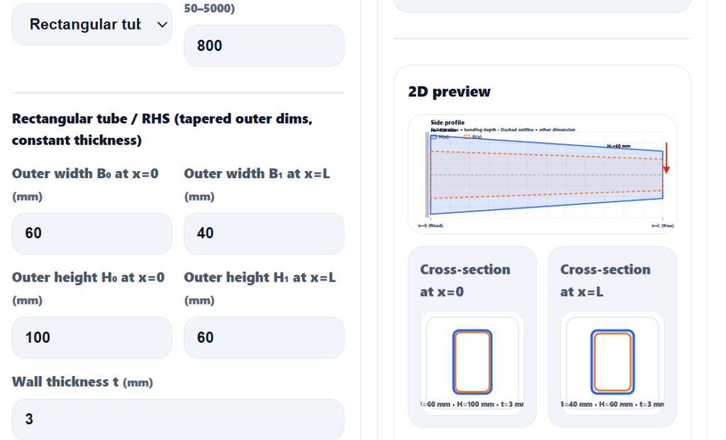
Then the last step is choosing the bending axis. I have per default chosen the Strong axis for all, even though if you have symmetric cross sections the Bending Axis’ are the the same.

This will now go through a sequence of calculations which i will explain in the Tapered Beam Calculator Explained Section, and give you the:

• Tip Deflection in mm
• Tip Rotation in mrad
• Equivalent tip stiffness in N/mm
• Volume in m^3
• Mass in kg
• Max bending stress at fixed end (assuming just elasticity)

This should be enough for you to not sit down and struggle with time consuming hand calculations. Although i reccomend sitting down and trying to do hand calculations to get a basis understanding of the procedure. That will in fact help you understand your specific configuration situation more within a Finite Element context later on, or simply to make sure that when you are designing something that people for example walk on, that you are not in doubt.

Tapered Beam Calculator Explained

In this section the Calculator will be explained. This is simply to document what has been done, and if anyone wants to recreate it, they can follow along these steps or simply just get a better understanding of calculations on a tapered beam.

Beam model and assumptions

The calculator uses classical Euler-Bernoulli beam theory under these assumptions:

• Small deflections and small rotations
• Linear elastic material with constant Young’s modulus E along the beam.
• Plane section remain plane (shear deformation is neglected)
• Bending about one chosen principal axis
• The beam is prismatic in material (constant density), but cross-sections can vary linearly along x.

Coordinate definition: x is measured from the fixed end (x=0) to the free end (x=L)

Inputs and units

Inputs are entered in mixed units but converted internally to SI:

• Length L in meters (m)
• Load P in newtons (N)
• Young’s modulus E in gigapascals (GPa) and converted to pascals (Pa)
• Density ρ in kg/m^3
• Geometric dimensions in millimeters (mm) and converted to meters (m)
• Integration slices N is dimensionless and controls numerical accuracy

Taper definition

Each geometric dimension is assumed to vary linearly from a start value at x=0 to an end value at x=L.

For any dimension a(x) with a0 at x=0 and a1 at x=L:

$$a(x)=a_0 + (a_1 – a_0) \cdot (\frac{x}{L})$$

Cross-Section properties

This is one of the difficult things about tapered beams which is that in the standard equation for a cantilever beam with a force at the free end is:

$$\delta_max = \frac{PL^3}{3EI}$$

Here for a cross section that is constant the second order area moment of inertia I is constant for both rotation axis. But with a tapered beam this is different. It is now a function of the length I(x). And the Cross sectional area also becomes a function of the length A(x). Together again with the Extreme-fiber distance which is constant for a fixed cross section, now it becomes a function of the distance, so c(x).

So,

For bending and weight calculations the calculator needs, at each x-position:

• Cross-sectional area A(x)
• Second order area moment of inertia I(x) about the chosen bending axis
• Extreme-fiber distance c(x) for bending stress at the fixed end (used at x=0)

Now i’m gonna explain how we can get these properties as a function of length split up for the different cross sections

Solid rectangle

Let b(x) be width and h(x) be height at position x.

Area:

$$ A(x)= b(x) \cdot h(x)$$

Second order area moment of inertia is for:

The strong axis

$$I(x)=b(x)\cdot \frac{h(x)^3}{12}$$

The weak axis

$$I(x)=h(x)\cdot \frac{b(x)^3}{12}$$

Solid circle

Let d(x) be diameter at position x.

Area:

$$ A(x) = \pi \cdot \frac{d(x)^2}{4} $$

Second order area moment of inertia:

$$ I(x) = \pi \cdot \frac{d(x)^4}{64} $$

Hollow circle (Pipe)

Let D(x) be outer diameter and t be the wall thickness (where the wall thickness is constant)

For the inner diameter we use a maximization function in the code:

$$ d(x) = max(0, D(x) – 2t) $$

The reason for this choice is for numerical stability, because if some input is very small near the end, then the inner diameter can become unstable. This is basically to save the calculator from exploding no matter what inputs come.

The Area is then:

$$ A(x) = \pi \cdot \frac{D(x)^2 – d(x)^2}{4} $$

The second order area moment of Inertia:

$$ I(x) = \pi \cdot \frac{D(x)^4 – d(x)^4}{64} $$

Rectangular hollow section (RHS)

Let B(x) be outer width and H(x) outer height, and t the wall thickness (constant along the length).

Inner dimensions are using maximizing functions again for numerical stability:

$$ B_i(x) = max(0, B(x) – 2t) $$

$$ H_i(x) = max(0, H(x) – 2t) $$

Area:

$$ A(x) = B(x) \cdot H(x) – B_i(x) \cdot H_i(x) $$

Second order area moment of inertia are given as:

Strong axis (about x-x, height is bending depth):

$$ I_{xx}(x) = \frac{B(x)\cdot H(x)^3 – B_i(x) \cdot H_i(x)^3}{12} $$

Weak axis (about y-y, width is bending depth):

$$ I_{yy}(x) = \frac{H(x)\cdot B(x)^3 – H_i(x) \cdot B_i(x)^3}{12} $$

Load case and bending moment

Since we only have one load case, which is a single point load P applied at the free end x=L for a cantilever, then we simply have this Bending moment along the beam:

$$ M(x) = P\cdot (L-x) $$

Deflection and rotation equations

Euler-Bernoulli curvature related the bending moment to deflection v(x). This equation is also known as the “Standard Beam differential equation”, which in my experience is used to solve for niche examples in terms of beams, but also all the standard equations you see in textbooks used at engineering jobs and workshops got derived using this equation:

$$ \frac{d^2v}{dx^2} = \frac{M}{E\cdot I} $$

And then inserting our dependacies of the length of the beam, because cross sections changes, we have:

$$ \frac{d^2v}{dx^2} = \frac{M(x)}{E\cdot I(x)} $$

To solve this equation and get the tip deflection and the tip rotation responses by integrating twice for the deflection and integrating once for the rotation. This results in the following:

$$v(L) = P\cdot \int_0^L \frac{(L-x)^2}{E\cdot I(x)}dx $$

And remembering that the rotation of a beam is defined as:

$$ \theta(x) = \frac{dv}{dx} $$

we get

$$\theta(L) = P\cdot \int_0^L \frac{(L-x)}{E\cdot I(x)}dx $$

As we can see this integral becomes a struggle to evaluate since we have two function of x in there, which would lead to a big struggle. This is why we will evaluate them numerically.

If we pull the constants out of the equation it results in us having two equations to numerically evaluate which we call J1 and J2:

$$J_1 = \int_0^L \frac{(L-x)}{I(x)}dx $$

$$J_2 = \int_0^L \frac{(L-x)^2}{I(x)}dx $$

then we have:

$$\theta(L)=\frac{P}{E}J_1, \quad v(L) =\frac{P}{E}J_2 $$

The next step is to discretize the beam into N slices

Discretization step

$$\text{For slice} \quad i = 0,1,…,N-1 $$

The midpoint is:

$$ x_i = (i+\frac{1}{2}) \Delta x $$

And why the midpoint you might ask? Well that’s because it is typically more accurate than using the left or right end of each slice, without beeing much more expensive.

The midpoint rule is defined as to approximate an integral as:

$$ \int_0^L f(x) dx \approx \sum_{i=0}^{N-1}= f(x_i) \cdot \Delta x $$

We use the same approach for the deflection integral, the rotation integral and the volume.

Note: If N is large, results change very little. If the section tapers sharply, you can increase N for stability.

Approximating each integral

Now for the exciting stuff, actually the computation and application of the numerical method

For the rotations integral we apply it such that:

$$J_1 = \int_0^L \frac{L-x}{I(x)}dx \approx \sum_{i=0}^{N-1}\frac{(L-x_i)}{I(x_i)} \Delta x $$

which equates to this equation for the rotation at x=L:

$$ \theta(L) \approx \frac{P}{E}\sum_{i=0}^{N-1}\frac{(L-x_i)}{I(x_i)} \Delta x $$

And for the deflection integral we have:

$$J_2 = \int_0^L \frac{(L-x)^2}{I(x)}dx \approx \sum_{i=0}^{N-1}\frac{(L-x_i)^2}{I(x_i)} \Delta x $$

Such that the deflection formulae becomes:

$$ v(L) \approx \frac{P}{E}\sum_{i=0}^{N-1}\frac{(L-x_i)^2}{I(x_i)} \Delta x $$

So this is exactly how we can evaluate the tapered beams deflection and curvature with a simple calculator. Just by applying the standard beam equation and the mid-point rule numerical method.

Volume and Mass Calculations

Since people also asked for a Tapered Beam weight calculator, i simply also implemented the midpoint-rule for approximating this accurately.

For the volume we have the following:

$$ V=\int_0^L A(x) dx \approx \sum_ {i=0}^{N-1} A(x_i) \Delta x $$

And then simply calculating the mass is:

$$ m = \rho V $$

What about the size of N?

So basically we need to choose the amount of slices in the discretization of the beam. The more the better, but the more computationally heavy it becomes.

The basic rules for this calculator, and in general for using numerical methods are to discretize more if you have sharper gradients. And what i mean by that in this tapered beam setting is, that if your pipe goes from 60mm to 10mm over a short length, then your second order area moment of inertia changes drastically.

And since the integrand contains

$$\frac{1}{I(x)}$$

then if I(x) becomes small everywhere suddenly, then it contributes to large deflections and rotations, and then we really need higher N.

I have tested the calculator though, and it doesn’t seem to hurt using N=10000, therefore i will take this as a learning step for example if you have singularity spots or sharp corners in a Finite Element context, then the same applies. You need a converged Mesh to evaluate your results and feel safe with them.

Finite element comparison of different cross sections

For good measure i did a simple finite element simulation in SolidWorks to compare with the calculator. I did this for all 4 cross sections, and compared tip displacements. I provided both screenshot of the calculator options, and a screenshot from the Finite element Analysis.

Solid rectangle comparison

For the Solid Rectangle i built the geometry in Solidworks, and used their Simulation tool to do the Finite elements analysis. It is just a Linear analysis.

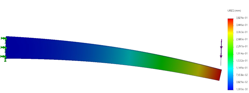
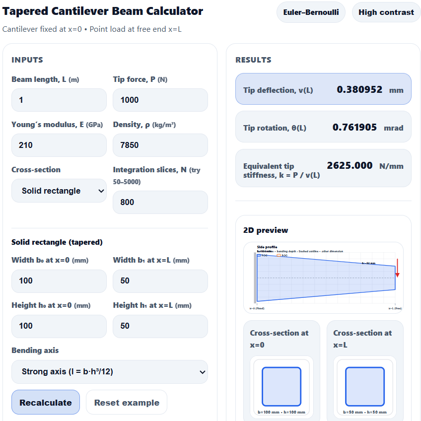
We can see that the tip end displacements are very close, but not exact:

$$v_{FEA,tip} \ne v_{calculator,tip} $$

$$0,3829mm \approx 0,3809mm $$

I have used a converged mesh (31821) quadratic elements. We can see that the results are similar, and that is nice, and shows that the calculator works.

Solid circle Comparison

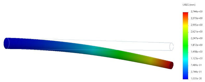
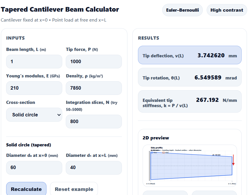
As we can see for this Solid circle comparison it is almost the same displacement as the tip with 8621 quadratic elements used:
$$3,744mm \approx 3,743mm $$

Hollow circle

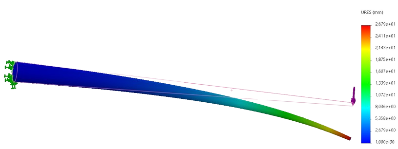
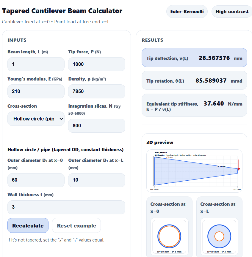
Here we can see a little difference of 0,2mm. Which is not that much. This tells us that the calculator is also good for the hollow circle. I used quadratic elements again… Its the same routine for all the analyses of the different cross-sections.

Rectangular Tube

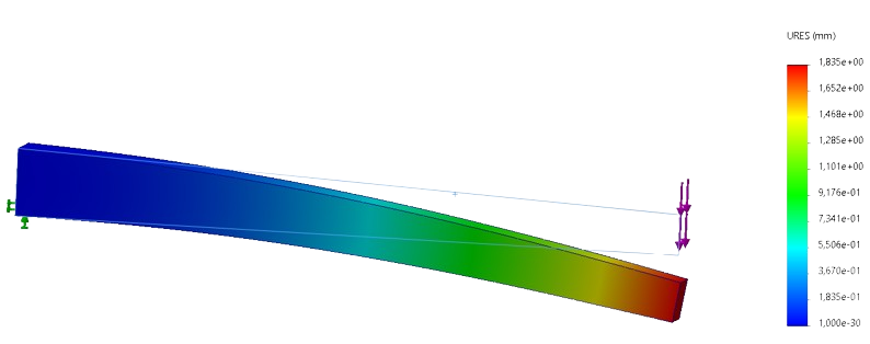
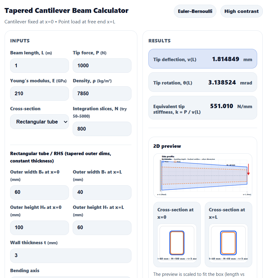
Once again the calculator is close here. Although here there is a difference of 0,021mm of displacement at the tip. But as a Calculator using numerical methods, and easy and quick to use it is very close! The amount of Elements used for this model was 34249 quadratic elements, just for good measure.

Round up

Overall i have established a well functioning and working tapered beam calculator, both for calculating the weight of tapered beams, but also the displacement at the end of a cantilever tapered beam with a load at the tip.

You can think of the whole process of building the calculator like this:

• The beam has been broken into N tiny beams
• At each tiny beam, we assume stiffness is constant and equal to the stiffness at its midpoint
• We add up the “small contributions” to rotations and deflection

The tapered beam calculator is a tool that is easy to use, it saves a lot of time for hand calculations, and it is faster than setting up a FE-model. Although it is an approximation. I really hope you enjoyed reading through and get good use out of the calculator for the future to come.